Building phylogeneric trees

Dmitry Kondrashov & Stefano Allesina Fundamentals of Biological Data Analysis – BIOS 26318

Goal

Let’s import some libraries:

library(ape) # most important library for phylogeny
library(phangorn) # tree reconstruction

Introduction

Darwin’s “I
think…”

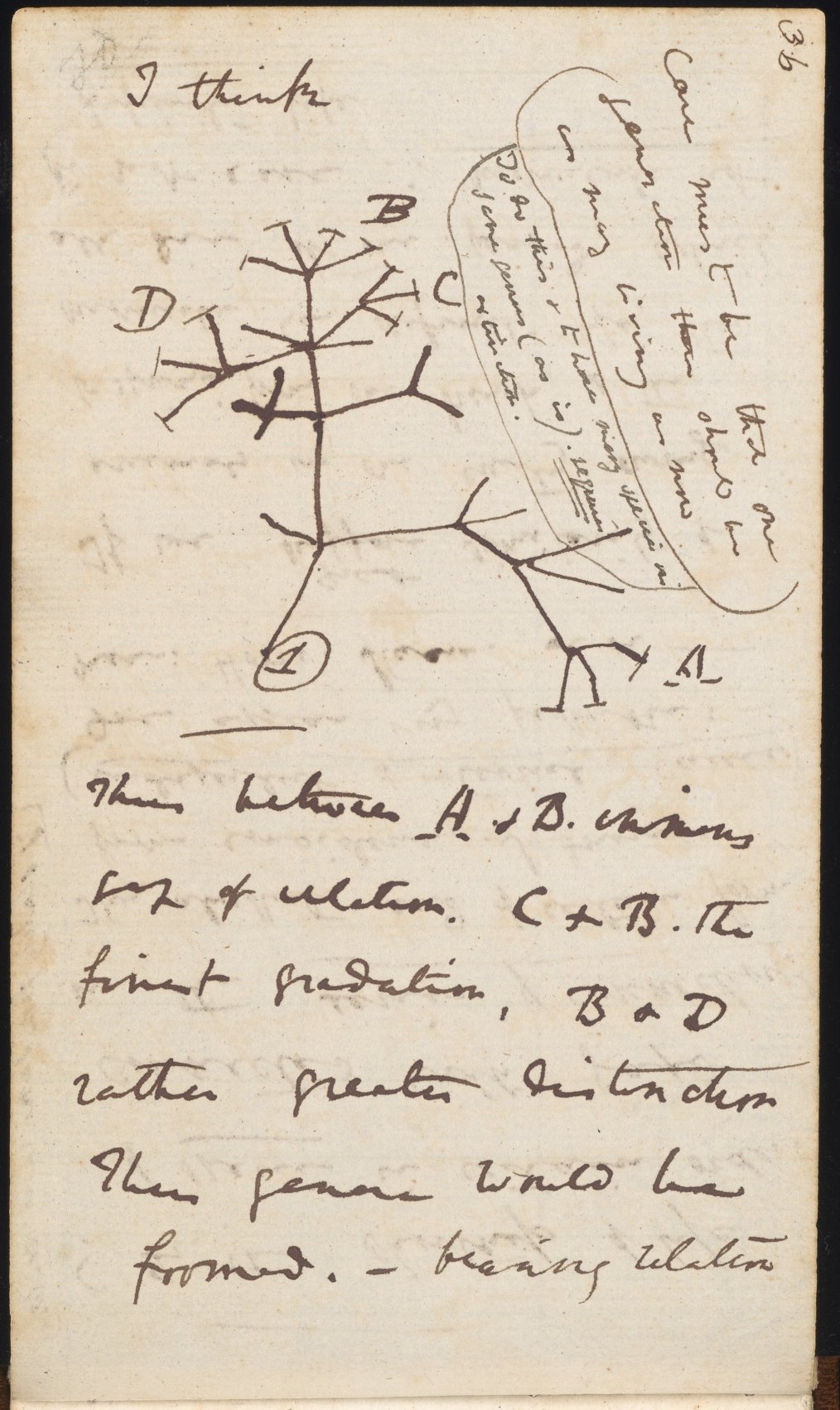
Since Darwin’s “I think” biologists have been constructing trees connecting species to their common ancestors. The goal of this brief tutorial is to introduce some of the basic terminology, and illustrate the most common approaches to building trees.

This tutorial is based on the freely available book The Mathematics of Phylogenetics, by Allman and Rhodes.

Input

The input is assumed to be a series of sequences, one for each taxon. For simplicity, we deal with DNA sequences, and assume that the taxa are different species. However, the methods introduced here can be extended to other types of sequences (e.g., amino acids, RNA, morphological features) and taxa (e.g., individuals of the same species, or even cells from the same individual). We assume the DNA sequences to be orthologous (i.e., to have descended from a common ancestral sequence) and to have been aligned (i.e., having many of the bases matching across the sequences for all the taxa).

DNA is composed of four nucleotides or bases: adenine (A), guanine (G), cytosine (C), and thymine (T). A and G are both purines, C and T are pyrimidines. When DNA is copied, small errors (mutations) can be introduced: we speak of substitutions when a base is changed, deletions when one or more consecutive bases are not copied, and insertions when new bases are introduced in the sequence. For this tutorial, we will concentrate on substitutions, which are believed to be the most common type of mutations. We distinguish between transition (from a purine to the other purine, or from pyrimidine to pyrimidine) and transversion (from one type to the other). Many models assume that transitions are more frequent than transversions (due to smaller changes in chemical stability of DNA).

Taxon	Sequence
Tax 1	ATTGCAATGGCA
Tax 2	ATTGCAATAGCA
Tax 3	ATTACAACGGCA
Tax 4	ATTACAACAGCA

Representing trees

A graph is a collection of vertices ( $V$ ) and edges ( $E$ ). We consider simple, undirected graph for most of the tutorial; simple means that self loops are not allowed and that each two nodes can be connected by one edge at most; undirected that we do not distinguish between $a \to b$ and $b \to a$ . A graph is connected if there is a way to go from any node to any other following its edges. A cycle is a closed path connecting a node to itself. A tree is a connected graph that contains no cycles.

We distinguish between rooted and unrooted trees: the root is a particular vertex from which all other taxa descend (the MRCA, most recent common ancestor of all taxa). Note that by placing the root in different places, we can obtain dramatically different-looking trees:

Unrooted and rooted
trees

Typically, we can only observe the tips or leaves of the tree (the extant species); their common ancestors are the internal nodes of the tree, which have to be inferred.

An unrooted tree with $n > 1$ leaves contains exactly $2n -2$ nodes, and $2n -3$ edges. A rooted tree has one extra node ( $2n -1$ ) and one extra edge ( $2n - 2$ ). There are very many trees one can form with $n$ leaves: we can count $(2n -3)!!$ rooted trees (where the double factorial becomes $1 \cdot 3 \cdot 5 \cdots (2n -3)$ ).

We can add a “length” to each edge, measuring how much change has accumulated between the two vertices. In case of “molecular clock” trees, we assume lengths to be measuring time, and all leaves have the same distance (computed summing the lengths along the branches) from the root. Trees in which all leaves have the same distance from the root are called ultrametric.

Ultrametric tree for 22
spiders

Mathematically, if we do not make an assumption of a “molecular clock” (i.e., that mutations are neutral and occurr at a predictable rate), we cannot identify the root of a tree without using extra information. Typically, what is done is to also align sequence(s) stemming from an outgroup, i.e., a taxon that is believed to be distantly related to the taxa we want to connect in our tree. Then, the root will connect the outgroup taxon with the rest of the tree.

Many of the methods for tree reconstruction are based on unrooted, unweighted trees, and a root and lengths can be determined once one has chosen a topology for the tree.

A simple way to represent a tree is provided by the Newick notation: the string (((a, b), c), (d, e)) represents a tree in which two nodes enclosed by parentheses are connected to a common ancestor (internal node). Note that the notation cannot readily discriminate among identical trees (e.g., ((d, e), (c, (b, a)))) so that spotting two identical trees is difficult to do by eye.

Building trees from sequence data

Provided with a set of orthologous, aligned sequences, we want to build a tree explaining the observed mutations. All methods to build trees from sequences are based on Occam’s razor: given alternative histories for the evolution of the sequences, take the “simplest” as the most probable.

Maximum Parsimony

Going back to our example:

Taxon	Sequence
Tax 1	ATTGCAATGGCA
Tax 2	ATTGCAATAGCA
Tax 3	ATTACAACGGCA
Tax 4	ATTACAACAGCA

we could think of the tree $((1, 2), (3, 4))$ that would be consistent with the changes in position 4 and 8; the changes in position 9, however, would require a further mutation for each branch. We can count the number of changes in the sequences required for each tree, and maximum parsimony can be summarized as “The best tree to infer from data is the one requiring the fewest changes”.

We can propose a tree, and for each edge connecting nodes $(u, v)$ , we can count the number of changes required to go from $u$ to $v$ . We can then sum all the changes (called the parsimony score) and choose the tree with the minimum score.

Example of parsimony
score

Computing the minimum score for a given tree and sequences for the leaves is called the “small parsimony problem” while computing the minimum parsimony over all trees is the “large parsimony problem”. The small problem can be solved efficiently (e.g., using the Fitch-Hartigan algorithm). The large problem is computationally very difficult.

Example: primates

# read alignement primates
fdir <- system.file("extdata/trees", package = "phangorn")
primates <- read.phyDat(file.path(fdir, "primates.dna"), format = "interleaved")
primates$Human

#   [1] 1 2 2 2 2 1 2 4 2 1 2 2 2 1 4 1 2 1 1 1 2 1 1 2 1 2 2 1 2 4 2 4 2 2 2 2 4
#  [38] 1 1 4 4 1 2 1 1 4 4 4 1 1 2 2 4 2 2 2 1 2 2 4 4 2 1 3 1 1 2 4 3 1 1 2 3 2
#  [75] 2 1 1 4 2 4 2 1 4 1 1 2 2 1 1 2 1 2 1 2 2 2 2 1 4 2 1 1 1 3 2 1 2 2 2 2 4
# [112] 2 2 1 1 2 1 2 1 2 2 2 3 2 1 2 1 2 2 4 2 2 1 2 2 2 2 2 2 4 2 3 4 2 4 1 2 3
# [149] 2 4 4 1 2 2 1 2 3 4 2 4 2 2 2 4 2 2 2 4 2 4 2 1 2 1 2 2 4 4 1 2 4 2 1 2 2
# [186] 4 4 2 4 2 2 2 1 1 1 2 3 1 2 4 4 2 3 2 1 2 2 1 2 1 1 2 3 2 2 1 2

Now let’s build a random tree and compute parsimony:

set.seed(0)
# generate random tree
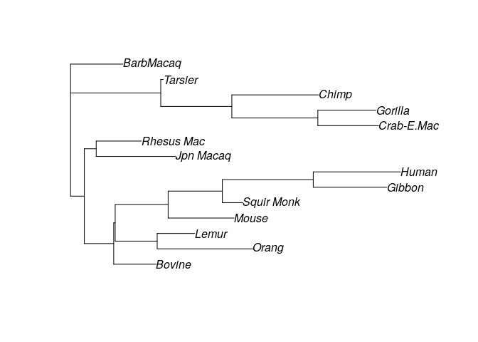
my_tree <- rtree(14, rooted = FALSE, tip.label = names(primates))
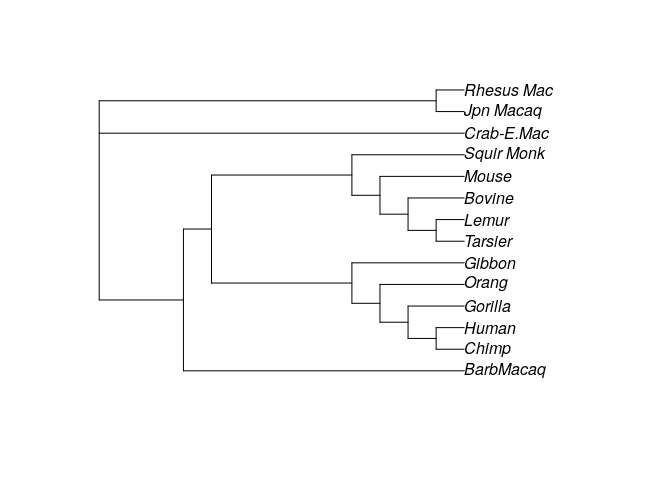
plot(my_tree)

We can compute the parsimony score for the tree:

parsimony(my_tree, primates)

# [1] 921

Meaning that to recover the observed sequences from the ancestral one, we need to assume 921 changes have occurred. Clearly, this doesn’t seem to be an especially promising tree (for example, Humans and Chimpanzees are quite far, while we know that they should be close). Let’s try with another random tree:

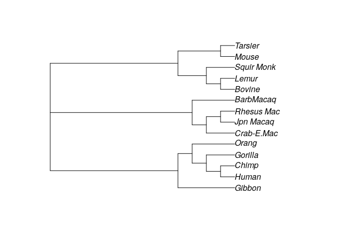
# try with another one
my_tree2 <- rtree(14, rooted = FALSE, tip.label = names(primates))
plot(my_tree2)

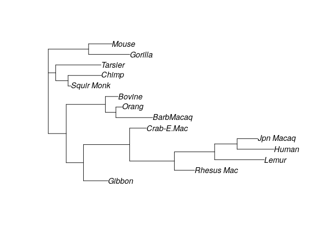
parsimony(my_tree2, primates)

# [1] 935

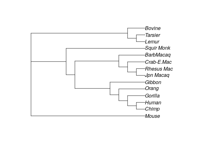
Which is even worse! We can try to “tweak” the structure of the tree to reduce the parsimony score by calling optim.parsimony. For example:

# try to find a good tree
optim_tree <- optim.parsimony(my_tree, primates)
plot(optim_tree)

# Final p-score 746 after  19 nni operations

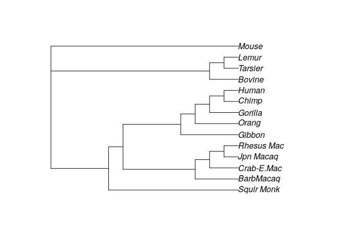
Trying with the other random tree:

optim_tree2 <- optim.parsimony(my_tree2, primates)
plot(optim_tree2)

# Final p-score 751 after  23 nni operations

This shows that the starting tree matters. In fact, we do not find especially good soltuions even after calling optim.parsimony. Now we are going to try again but with a starting tree based on distances (explained below).

# compute distances
dm <- dist.ml(primates)
# build tree using distances
treeNJ <- NJ(dm)
treeUPGMA <- upgma(dm)
parsimony(treeNJ, primates)
optim_tree3 <- optim.parsimony(treeNJ, primates)
plot(optim_tree3)

parsimony(treeUPGMA, primates)
optim_tree4 <- optim.parsimony(treeUPGMA, primates)
plot(optim_tree4)

# [1] 746
# Final p-score 746 after  0 nni operations 
# [1] 751
# Final p-score 746 after  1 nni operations

`#ParsimonyGate`

Maximum parsimony is often used, but has several problems (in fact, no method is perfect, and each has strengths and limitations). For example, there typically exist several trees with the same score.

The journal Cladistics published an editorial in February 2016 stating that “Phylogenetic data sets submitted to this journal should be analysed using parsimony. If alternative methods give different results and the author prefers an unparsimonious topology, he or she is welcome to present that result, but should be prepared to defend it on philosophical grounds” (emphasis mine). The mention of phylosophy to justify scientific results led to a twitter storm, ignited by Jonathan Eisen (for an entertaining account, see here).

Distance Methods

A second class of methods is based on measuring “dissimilarity” (or “distance”) between sequences. The idea is then to preferentially connect with a common ancestors species that are “close”. This is similar to what we’ve done with MDS, and the basic notion of distance is the same. We start by computing a matrix of dissimilarities (or distances), and then use an algorithm to build a tree.

A simple method to build a tree given the dissimilarity matrix is called unweighted pair-group method with arithmetic means (UPGMA). The idea is very simple: we start by joining the two leaves that have the smallest distance. We then remove the leaves and add a new node that is the average between the two leaves. We then repeat the same operation until we have built the tree.

UPGMA in
action

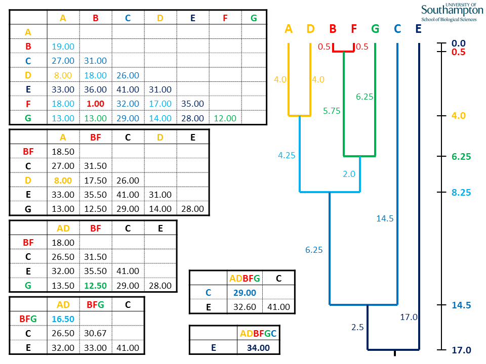
Note that the UPGMA builds trees with branch lengths and assumes that the data are produced by a molecular clock. Because this condition is often violated, we need to choose another algorithm whenever we suspect the dissimilarities are not stemming from an ultrametric tree. In practice, the “Neighbor Joining” algorithm (NJ) is often used.

The algorithm is based on the so-called four-point condition: given four taxa $a, b, c, d$ (which might include repetitions), in a metric tree we have

$\delta(a, b) + \delta(c, d) \leq \max\{\delta(a, c) + \delta(b, d), \delta(a, d) + \delta(b, c)\}$
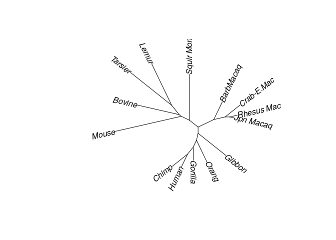
This inequality is used to choose with two leaves to join, and the process is repeated as in UPGMA. Despite being more complex, NJ is often used in practice to produce a good starting tree. Note that NJ builds an unrooted tree.

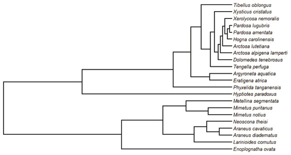
plot(treeNJ, type = "unrooted", lab4ut = "axial")

Likelihood based methods

The goal of likelihood-based methods is to compute a probability of having observed a given set of sequences given a tree. To do so, we often make a strong assumption of independence: each site behaves independently, and the bases are taken from the same distribution (i.i.d.).

Because of this assumption, we do not care of the exact sequence, only of the number of bases of each kind. For example, we can assume that the root distribution vector is

$p_\rho = (p_A, p_G, p_C, p_T)$

with elements summing to one.

Now we can model the probability that a base in the root will mutate to another base by substitution along an edge $e$ . We can use a transition matrix (or Markov matrix):

$M_e = \begin{pmatrix} p_{AA} & p_{AG} & p_{AC} & p_{AT}\\ p_{GA} & p_{GG} & p_{GC} & p_{GT}\\ p_{CA} & p_{CG} & p_{CC} & p_{CT}\\ p_{TA} & p_{TG} & p_{TC} & p_{TT} \end{pmatrix}$

with nonnegative entries and rows summing to one. This matrix encodes the probability that a base in the ancestor was substituted in the descendant along edge $e$ . But how can we compute the matrix for a given edge?

Clearly, each edge could give rise to its own Markov matrix, making it difficult to infer a tree from sequences. Instead, we can link all the matrices along all edges by making them all a function of a matrix of rates and the length of the edge. The solution is to build a matrix of rates $Q$ (with rows summing to zero, and off-diagonal elements that are positive). The elements of the matrix $Q$ describe the instantaneous rate of substitution. We then want to model the time elapsed along one edge. We solve the differential equation:

$\frac{d p(t)}{dt} = p(t) Q$

Because it is a linear system of ODEs:

$p(t) = p(0) e^{Qt} = p(0) S e^{\Lambda t} S^-1$

where $S$ is the matrix of eigenvectors, and $\Lambda$ the diagonal matrix of eigenvalues of $Q$ .

When we have an edge $e$ with corresponding time $t_e$ , we choose $M_e = M(t_e) = e^{Qt_e}$ to be the matrix projecting the proportion of bases in the ancestor to the number of bases in the descendent. In practice, out of computational convenience, often we choose $Q$ with a very special structure.

Jukes-Cantor Model

This is the simplest model for base substitution. It assumes that in the ancestral sequence, all bases occurr with the same probability:

$p_\rho = (1/4, 1/4, 1/4, 1/4)$
and that each base is substituted by any other with equal rates:

$Q = \begin{pmatrix} -\alpha & \alpha / 3 & \alpha / 3 & \alpha / 3 \\ \alpha / 3 & -\alpha & \alpha / 3 & \alpha / 3 \\ \alpha / 3 & \alpha / 3 & -\alpha & \alpha / 3 \\ \alpha / 3 & \alpha / 3 & \alpha / 3 & -\alpha \end{pmatrix}$
As such, the total rate at which a specific base is substituted (by any of the other three) is $\alpha$ . With some calculation, we find that:

$S = \begin{pmatrix} 1 & 1 & 1 & 1 \\ 1 & -1 & 1 & -1 \\ 1 & 1 & -1 & -1 \\ 1 & -1 & -1 & 1 \end{pmatrix}$
and

$\Lambda = \begin{pmatrix} 0 & 0 & 0 & 0\\ 0 & -\frac{4}{3} \alpha & 0 & 0\\ 0 & 0 & -\frac{4}{3} \alpha & 0\\ 0 & 0 & 0 & -\frac{4}{3} \alpha\\ \end{pmatrix}$

and as such:

$M(t) = e^{Qt} = S e^{\Lambda t} S^{-1} = \begin{pmatrix} 1- a(t) & a(t) / 3 & a(t) / 3 & a(t) / 3 \\ a(t) / 3 & 1 -a(t) & a(t) / 3 & a(t) / 3 \\ a(t) / 3 & a(t) / 3 & 1 -a(t) & a(t) / 3 \\ a(t) / 3 & a(t) / 3 & a(t) / 3 & 1-a(t) \end{pmatrix}$

where $a(t) = \frac{3}{4}\left(1 - e^{-\frac{4}{3} \alpha t}\right)$ . Clearly, the larger the $t$ or the $\alpha$ , the more substitutions we expect to occurr. Note however that the model encodes a stable base distribution at all vertices of the tree: $p_\rho M(t) = p_\rho$ .

Other models

Other models use a larger number of parameters, attempting to model mutations more precisely. For example, the Kimura 2-parameter model uses the matrix:

$Q = \begin{pmatrix} -\beta - 2 \gamma & \beta & \gamma & \gamma \\ \beta & -\beta - 2 \gamma & \gamma & \gamma \\ \gamma & \gamma & -\beta - 2 \gamma & \beta \\ \gamma & \gamma & \beta & -\beta - 2 \gamma\\ \end{pmatrix}$

Which can be treated in the same way as above, leading to a 2-parameter $M(t)$ .

Maximum likelihood

Armed with the definitions above, we now want to fit a length of an edge stemming from the root. We have sequences $S0$ and $S1$ , and we build the matrix $N$ whose elements $n_{ij}$ counts the number of bases that were of type $i$ in the ancestral state, and $j$ in the descendant.

For example:

$S0: ATTACGGTT$

$S1: AAGGTCGTT$

Then the matrix $N$ (the order is always AGCT) becomes:

$N = \begin{pmatrix} 1 & 1 & 0 & 0 \\ 0 & 1 & 1 & 0 \\ 0 & 0 & 0 & 1 \\ 1 & 1 & 0 & 2 \end{pmatrix}$

We want to know what is the maximum likelihood estimate for the time between $S0$ and $S1$ given a model.

For example, if we choose the Jukes-Cantor model, we have that we assume $p_0 = (1/4, 1/4, 1/4, 1/4)$ , and the probabilities of observing a given transition would be:

$P(t) = \text{diag}(p_0) M(t) = \begin{pmatrix} (1- a(t)) / 4 & a(t) / 12 & a(t) / 12 & a(t) / 12 \\ a(t) / 12 & (1 -a(t)) / 4 & a(t) / 12 & a(t) / 12 \\ a(t) / 12 & a(t) / 12 & (1 -a(t))/4 & a(t) / 12 \\ a(t) / 12 & a(t) / 12 & a(t) / 12 & (1-a(t)) / 4 \end{pmatrix}$

The likelihood of a given edge length, $t$ would be:

$L(t \vert N ) = \prod_{i,j} p_{ij}^{n_{ij}}$

Taking the log-likelihood:

$\log L(t \vert N ) = \sum_{i,j} {n_{ij} \log p_{ij}} = \log(a / 12) \sum_{j\neq i} n_{ij} + \log((1-a) / 4) \sum_i n_{ii}$

Taking the derivative with respect to $t$ , setting it to zero, and massaging the equation we obtain:

$a(\hat{t}) = \frac{\sum_{j\neq i} n_{ij}}{\sum_{j, i} n_{ij}}$

For example, for the matrix above $a(\hat{t}) = 5/9$ . Because $a(t) = 3/4 (1 - e^{(-t 4/3)})$ , we get $\hat{t} \approx 1.0124$ , setting the maximul likelihood estimate for the length of the branch.

Using this method, we can find the maximum likelihood estimate for all the branches of a tree. We can then propose a tree, and then compute the product of all likelihoods. Given that there are many possible trees, we need a smart way to explore the space. The algorithm by Felsenstein (1981, Evolutionary trees from DNA sequences: a maximum likelihood approach) was the first to allow an efficient search of the space of trees, and the first to propose the method above to find optimal branch lengths.

Compute using a Jukes-Cantor model:

# compute likelihoods
test_NJ <- pml(treeUPGMA, data=primates, model = "JC")
print(test_NJ)

# 
#  loglikelihood: -3079.976 
# 
# unconstrained loglikelihood: -1230.335 
# 
# Rate matrix:
#   a c g t
# a 0 1 1 1
# c 1 0 1 1
# g 1 1 0 1
# t 1 1 1 0
# 
# Base frequencies:  
# 0.25 0.25 0.25 0.25

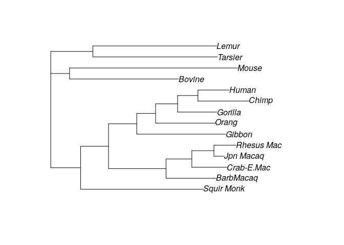
Try optimizing by allowing changes in topology:

fitJC <- optim.pml(test_NJ, data=primates,
                    rearrangement = "NNI")
print(fitJC)
plot(fitJC)

# optimize edge weights:  -3079.976 --> -3070.765 
# optimize edge weights:  -3070.765 --> -3070.764 
# optimize topology:  -3070.764 --> -3068.417 
# optimize topology:  -3068.417 --> -3068.295 
# optimize topology:  -3068.295 --> -3068.295 
# 2 
# optimize edge weights:  -3068.295 --> -3068.295 
# optimize topology:  -3068.295 --> -3068.295 
# 0 
# optimize edge weights:  -3068.295 --> -3068.295 
# 
#  loglikelihood: -3068.295 
# 
# unconstrained loglikelihood: -1230.335 
# 
# Rate matrix:
#   a c g t
# a 0 1 1 1
# c 1 0 1 1
# g 1 1 0 1
# t 1 1 1 0
# 
# Base frequencies:  
# 0.25 0.25 0.25 0.25

Bayesian methods

These methods can be extended to include priors. We can use a flat prior for the ancestral sequence, for the base substitution model, and over the space of possible trees and, via MCMC, construct the posterior distribution for all the parameters. The hope is to find strong support (i.e., posterior probability close to one) for a single tree; alternatively, many trees with high posterior can be summarized in a consensus tree.