Example: Homophily in authorship
Stefano Allesina QuEST Workshop, U. Vermont, Apr 2021
Introduction
We want to test whether authors are more likely to collaborate with other authors of the same sex. To test this idea, we use the probability that the first (last) author was assigned a certain sex at birth, computed as the frequency of a certain name/sex combination in the data from the Social Security Administration.
Data
We take all the articles for which we have an estimate of the probability that the first author and the last author are female. Importantly, we exclude papers with only a single author, as in those cases the first and last authors are the same person!
library(tidyverse)
dt <- read_csv("../data/plos_compbio.csv")
# filter data
dt2 <- dt %>%
  filter(document_type == "Article") %>%
  filter(!is.na(first_au_F), !is.na(last_au_F)) %>%
  filter(!is.na(num_authors)) %>% filter(num_authors > 1)
As you can see, the data contain various combinations (including the “corners” M/M, M/F, F/M, F/F):
pl1 <- ggplot(dt2) +
  aes(x = first_au_F, y = last_au_F) +
  geom_point(alpha = 0.1) +
  theme_bw()
show(pl1)
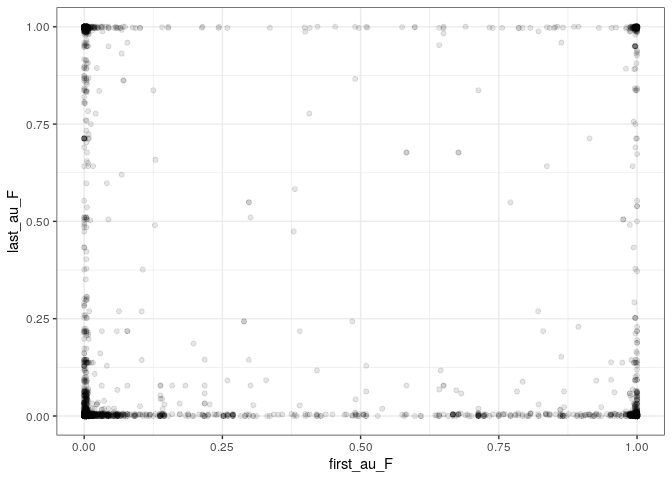
Note also that we have more density close to (0, 0), (0, x) and (x, 0), consistently with the fact that the number of women first/last authors has been increasing, but is still below that of men.
Strategy 1: correlation + randomization
We compute the correlation between first_au_F and last_au_F, then
repeatedly randomize the data and check whether the observed correlation
is higher than
expected:
compute_corr_authors <- function(x) return(cor(x$first_au_F, x$last_au_F))
observed <- compute_corr_authors(dt2)
num_randomizations <- 5000
randomized <- sapply(1:num_randomizations, function(x) {
  tmp <- dt2 %>% mutate(first_au_F = sample(first_au_F))
  return(compute_corr_authors(tmp))
  })
Now plot and compute a p-value
pl2 <- ggplot(data = tibble(correlation = randomized)) + aes(x = correlation) +
  geom_histogram(binwidth = 0.005, fill = "azure2", colour = "black") +
  geom_vline(xintercept = observed, colour = "red") +
  theme_bw()
show(pl2)
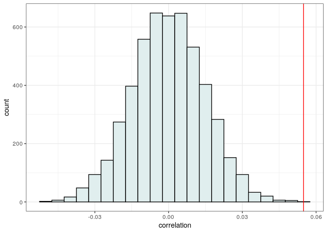
print("p(observed <= randomized)")
print(sum(observed <= randomized) / length(randomized))
# [1] "p(observed <= randomized)"
# [1] 2e-04
Showing that the correlation is positive, and higher than what expected.
Strategy 2: correlation + randomization on transformed data
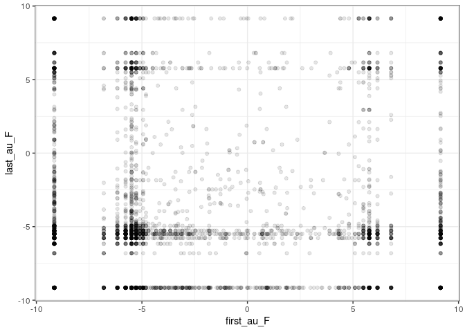
Proportions/probabilities are a bit tricky to work with—typically we want to transform the data prior to computing a correlation. A commonly employed strategy is to analyze the log-odds-ratio (as in the logistic regression)—which however requires not to have “pure” zeros or ones in the data set. We can “compress” the data using the approach by Smithson and Verkuilen’s[1] and then log-transform the odds ratios:
compress_01 <- function(x){
   # Smithson and Verkuilen's (2006) formula
   return((x * (length(x) - 1) + 0.5) / length(x))
}

logit_transform <- function(x){
  # transform proportions x' = log(x/(1-x))
  return(log(x / (1 - x)))
}

dt3 <- dt2 %>% mutate(first_au_F = logit_transform(compress_01(first_au_F)),
                      last_au_F = logit_transform(compress_01(last_au_F)))
pl1t <- ggplot(dt3) +
  aes(x = first_au_F, y = last_au_F) +
  geom_point(alpha = 0.1) +
  theme_bw()
show(pl1t)
Repeating the procedure, we find the same qualitative result:
compute_corr_authors <- function(x) return(cor(x$first_au_F, x$last_au_F))
observed <- compute_corr_authors(dt3)
num_randomizations <- 5000
randomized <- sapply(1:num_randomizations, function(x) {
  tmp <- dt3 %>% mutate(first_au_F = sample(first_au_F))
  return(compute_corr_authors(tmp))
  })
Now plot and compute a p-value
pl3 <- ggplot(data = tibble(correlation = randomized)) + aes(x = correlation) +
  geom_histogram(binwidth = 0.005, fill = "azure2", colour = "black") +
  geom_vline(xintercept = observed, colour = "red") +
  theme_bw()
show(pl3)
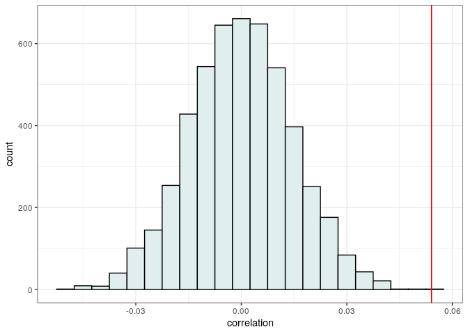
print("p(observed <= randomized)")
print(sum(observed <= randomized) / length(randomized))
# [1] "p(observed <= randomized)"
# [1] 0
Strategy 3: hard assignment + randomization
Alternatively, we can assign F to authors with first_au_F larger
than an arbitrary cutoff (here, 0.95), and count the number of pairs
F/F in the observed and randomized
data:
dt2 <- dt2 %>% mutate(first_gender = ifelse(first_au_F > 0.95, "F", "M/U"),
                      last_gender = ifelse(last_au_F > 0.95, "F", "M/U"))
count_FF <- function(tmp) {
  return(nrow(tmp %>% filter(first_gender == "F", last_gender == "F")))
}
observed <- count_FF(dt2)
num_randomizations <- 5000
randomized <- sapply(1:num_randomizations, function(x) {
  tmp <- dt2 %>% mutate(first_gender = sample(first_gender))
  return(count_FF(tmp))
  })
Again, we find the same qualitative result:
pl4 <- ggplot(data = tibble(FF_papers = randomized)) + aes(x = FF_papers) +
  geom_histogram(binwidth = 5, fill = "azure2", colour = "black") +
  geom_vline(xintercept = observed, colour = "red") +
  theme_bw()
show(pl4)
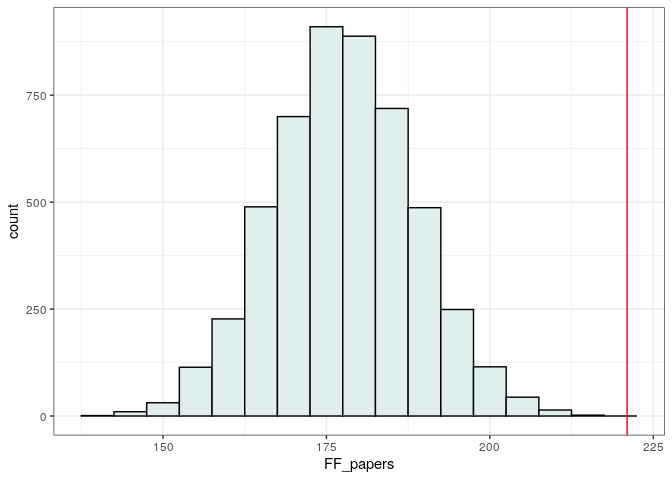
print("p(observed <= randomized)")
print(sum(observed <= randomized) / length(randomized))
# [1] "p(observed <= randomized)"
# [1] 0
Conclusions
Authors tend to co-author papers with authors of the same sex more often than what expected by chance. Previous studies have found that homophily extends well beyond sex[2].
-
A better lemon squeezer? Maximum-likelihood regression with beta-distributed dependent variables, Psychol Methods. 2006
-
Gallivan & Ahuja (2015) Co-authorship, homophily, and scholarly influence in information systems research. Journal of the Association for Information Systems; Ghiasi et al. (2018) Gender homophily in citations. 3rd International Conference on Science and Technology Indicators; Wang et al. Gender-based homophily in collaborations across a heterogeneous scholarly landscape. arXiv