source("skwara_et_al_2022.R")GLV and experimental data — Hands on tutorial
Data
For our explorations, we are going to use recent data from Ishizawa and colleagues, which you can find here:
H. Ishizawa, Y. Tashiro, D. Inoue, M. Ike, H. Futamata. Learning beyond-pairwise interactions enables the bottom–up prediction of microbial community structure PNAS 121 (7) e2312396121 (2024).
The Authors inoculated duckweed (Lemna minor) with synthetic bacterial communities formed by all possible combinations of seven strains. To this end, they cultured the infected duckweed in flasks for 10 days. At the end of the experiment, they plated the communities on agar plates containing antibiotics that would allow the growth only of a particular strain. In this way, they were able to measure the final density of each of the seven strains in each of the \(2^7 - 1 = 127\) possible communities, and conducted each experiment in replicate. The full data set reports the outcome of 692 separate experiments!
More modestly, here we are going to focus on a smaller pool of three strains taken from the seven available. We therefore have \(7\) possible communities, ranging from a single strain growing in isolation to the three strains growing together.
Here’s the full table:
| DW067 | DW102 | DW145 |
|---|---|---|
| 0.8 | ||
| 0.812 | ||
| 0.858 | ||
| 0.874 | ||
| 0.854 | ||
| 0.951 | ||
| 0.823 | ||
| 0.922 | ||
| 1 | ||
| 0.529 | ||
| 0.356 | ||
| 0.532 | ||
| 0.409 | ||
| 0.416 | ||
| 0.548 | ||
| 0.645 | ||
| 0.41 | ||
| 0.367 | ||
| 0.663 | 0.604 | |
| 0.703 | 0.909 | |
| 0.395 | 0.661 | |
| 0.54 | 0.487 | |
| 0.919 | 0.981 | |
| 0.707 | 0.828 | |
| 0.729 | ||
| 0.781 | ||
| 0.811 | ||
| 1 | ||
| 0.811 | ||
| 0.793 | ||
| 0.617 | ||
| 0.919 | ||
| 0.645 | ||
| 0.513 | 0.719 | |
| 0.419 | 0.428 | |
| 0.432 | 0.546 | |
| 0.197 | 0.598 | |
| 0.249 | 0.904 | |
| 0.242 | 0.558 | |
| 0.541 | 0.563 | |
| 0.568 | 0.755 | |
| 0.371 | 0.707 | |
| 0.566 | 0.524 | |
| 0.839 | 0.433 | |
| 0.796 | 0.609 | |
| 0.328 | 1 | 0.416 |
| 0.321 | 0.436 | 0.58 |
| 0.378 | 0.57 | 0.381 |
| 0.386 | 0.602 | 0.563 |
| 0.379 | 0.774 | 0.293 |
We can therefore associated each measurement with a) the strain being measured, \(i\); b) the community in which \(i\) was grown, \(k\); and c) the (biological) replicate experiment, \(r\).
Loading the code
We are going to use the code accompanying the paper
- Skwara, A., Lemos‐Costa, P., Miller, Z.R. and Allesina, S., 2023. Modelling ecological communities when composition is manipulated experimentally. Methods in Ecology and Evolution, 14(2), pp.696-707.
which you can find here
https://github.com/StefanoAllesina/skwara_et_al_2022/
we have slightly massaged the code for this tutorial.
To load the code in R change to the directory where you have stored the tutorial, and source this code:
Sum of squares
First, we are going to use all the data to find a matrix \(B\) that best encodes the density of the populations. To this end, we try to minimize the SSQ
\[ SSQ(B) = \sum_r \sum_k \sum_i \left(\tilde{x}^{(k,r)}_i - x^{(k)}_i \right)^2 \]
This can be accomplished by calling:
full_SSQ <- run_model(
  datafile = "Ishizawa_3_strains.csv", # csv file containing the data to be fit
  model = "full", # estimate B allowing each coefficient to take the best value
  goalf = "SSQ", # minimize Sum of Squared Deviations
  pars = NULL, # start from Identity matrix
  skipEM = TRUE, # go directly to numerical optimization
  plot_results = TRUE # plot the results
)
`mutate_if()` ignored the following grouping variables:
• Column `comm`[1] "numerical search"
[1] 1.289597
[1] 1.289597
[1] 1.289597
[1] 1.289597
[1] 1.289597
[1] 1.289597
[1] 1.289597
[1] 1.289597
[1] 1.289597
[1] 1.289597
The values being printed are the SSQ after each round of numerical optimization (in this case, the calculation converges immediately to the solution).
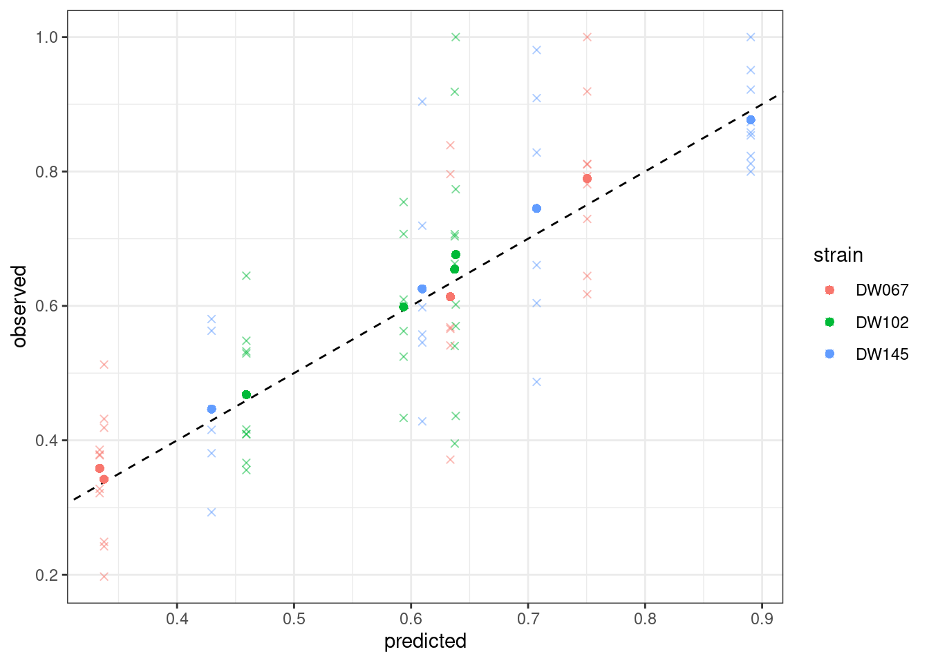
The boxplots show the data (points), as well as the corresponding boxplots, with the horizontal line being the median value of \(\tilde{x}_i^{(k,r)}\) across \(r\), the triangle shows the location of the empirical mean. The circle marks the fitted mean value for the combination of strain/community, obtained computing \(\left(B^{(k,k)}\right)^{-1}1_{\|k\|}\). As you can see, we can find a matrix \(B\) that recapitulates the observed means quite well.
The variable \(full_SSQ\) now contains:
glimpse(full_SSQ)List of 8
$ data_name : chr "Ishizawa_3_strains"
$ observed : num [1:50, 1:3] 0 0 0 0 0 0 0 0 0 0 ...
..- attr(*, "dimnames")=List of 2
.. ..$ : NULL
.. ..$ : chr [1:3] "DW067" "DW102" "DW145"
$ predicted : num [1:50, 1:3] 0 0 0 0 0 0 0 0 0 0 ...
..- attr(*, "dimnames")=List of 2
.. ..$ : NULL
.. ..$ : chr [1:3] "DW067" "DW102" "DW145"
$ variances : num [1:50, 1:3] 0 0 0 0 0 0 0 0 0 0 ...
..- attr(*, "dimnames")=List of 2
.. ..$ : NULL
.. ..$ : chr [1:3] "DW067" "DW102" "DW145"
$ B : num [1:3, 1:3] 1.3 -0.479 0.875 0.246 2.143 ...
$ pars : num [1:9] 1.63166 0.02719 -1.28356 -0.00694 0.43581 ...
$ goal_function: num 1.29
$ goal_type : chr "SSQ"Let’s plot the predicted vs. observed values:
plot_pred_obs(full_SSQ)
Where the points mark the predicted vs observed means, and the crosses the full data. The dashed line is the 1:1 line.
Weighted leas squares
We can repeat the calculation, but this time trying to minimize
\[ WLS(B) = \sum_r \sum_k \sum_i \left(\frac{\tilde{x}^{(k,r)}_i - x^{(k)}_i}{\sigma^{(k)}_i} \right)^2 \]
by calling:
full_WLS <- run_model(
  datafile = "Ishizawa_3_strains.csv", # csv file containing the data to be fit
  model = "full", # estimate B allowing each coefficient to take the best value
  goalf = "WLS",
  pars = NULL, # start from Identity matrix
  skipEM = TRUE, # go directly to numerical optimization
  plot_results = TRUE # plot the results
)
`mutate_if()` ignored the following grouping variables:
• Column `comm`[1] "numerical search"
[1] 67.07833
[1] 67.07833
[1] 67.07833
[1] 67.07833
[1] 67.07833
[1] 67.07833
[1] 67.07833
[1] 67.07833
[1] 67.07833
[1] 67.07833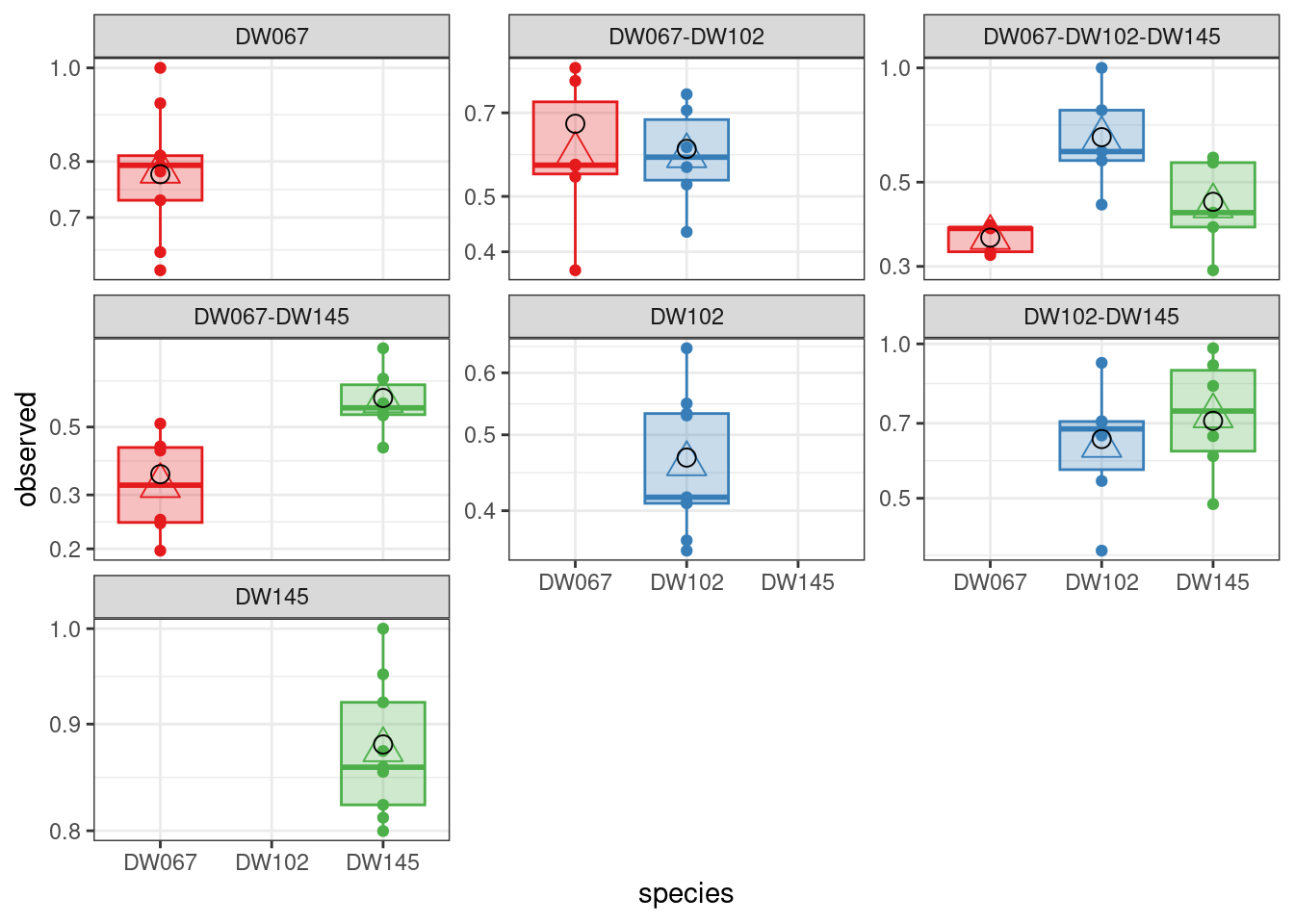
plot_pred_obs(full_WLS)
Notice that the points have moved slightly—this is because we are penalizing deviations differently depending on the measured variance (and thus points with a higher variance can depart more strongly from the 1:1 line).
Maximum likelihood
Now we take a different approach, and take the observations to be independent samples from a log-normal distribution:
\[ \tilde{x}_i^{(k,r)} \sim LN(x_i^{(k)}, \sigma_i) \]
i.e., we take each variable to have a mean determined by the corresponding \(x_i^{(k)}\), and a variance parameter that depends only on strain identity.
full_LN <- run_model(
  datafile = "Ishizawa_3_strains.csv", # csv file containing the data to be fit
  model = "full", # estimate B allowing each coefficient to take the best value
  goalf = "LikLN",
  pars = NULL, # start from Identity matrix
  skipEM = TRUE, # go directly to numerical optimization
  plot_results = TRUE # plot the results
)
`mutate_if()` ignored the following grouping variables:
• Column `comm`[1] "numerical search"
[1] -49.19108
[1] -49.19108
[1] -49.19108
[1] -49.19108
[1] -49.19108
[1] -49.19108
[1] -49.19108
[1] -49.19108
[1] -49.19108
[1] -49.19108
plot_pred_obs(full_LN)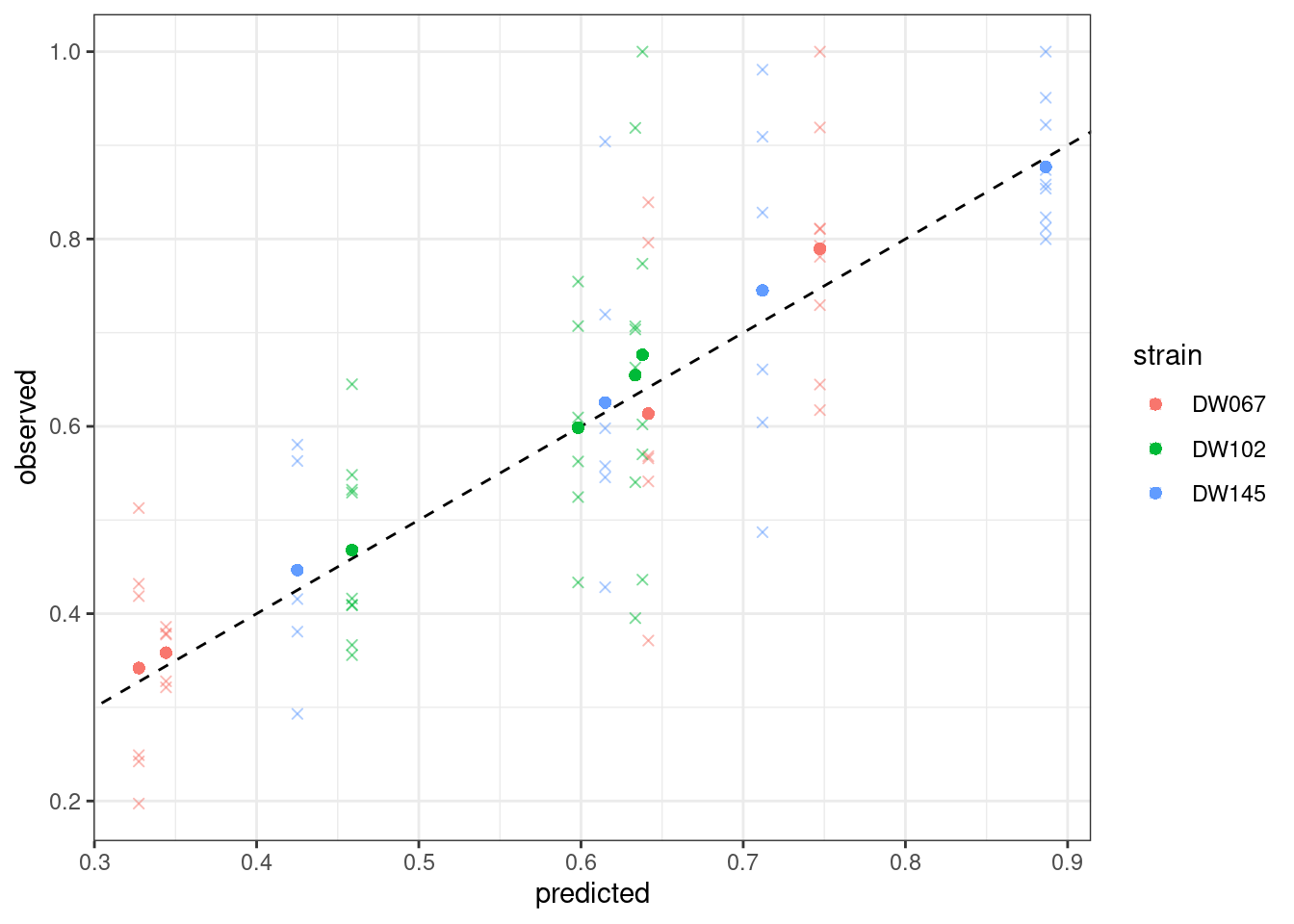
Also in this case, we obtain a good fit.
Leave-one-out cross validation
The ultimate test for this type of model is to be able to predict experimental results before running the experiment.
In our case, we can try to leave out one of the 7 communities, and see which model recover the best result:
dt <- read_csv("Ishizawa_3_strains.csv")Rows: 50 Columns: 3
── Column specification ────────────────────────────────────────────────────────
Delimiter: ","
dbl (3): DW067, DW102, DW145
ℹ Use `spec()` to retrieve the full column specification for this data.
ℹ Specify the column types or set `show_col_types = FALSE` to quiet this message.# the last row contains an experiment with only DW067 and DW102
dt %>% slice(40)# A tibble: 1 × 3
DW067 DW102 DW145
<dbl> <dbl> <dbl>
1 0.541 0.563 0LOO_LN <- run_model_LOO(datafile = "Ishizawa_3_strains.csv", model = "full", goalf = "LikLN", pars = NULL, skipEM = TRUE, plot_results = TRUE,
LOO_row_num = 40 # exclude all experiments with this community
)`mutate_if()` ignored the following grouping variables:
• Column `comm`[1] "numerical search"
[1] -43.08928
[1] -43.08928
[1] -43.08928
[1] -43.08928
[1] -43.08928
[1] -43.08928
[1] -43.08928
[1] -43.08928
[1] -43.08928
[1] -43.08928
LOO_WLS <- run_model_LOO(datafile = "Ishizawa_3_strains.csv", model = "full", goalf = "WLS", pars = NULL, skipEM = TRUE, plot_results = TRUE,
                        LOO_row_num =  40 # exclude all experiments with this community
)
`mutate_if()` ignored the following grouping variables:
• Column `comm`[1] "numerical search"
[1] 56.05198
[1] 56.05198
[1] 56.05198
[1] 56.05198
[1] 56.05198
[1] 56.05198
[1] 56.05198
[1] 56.05198
[1] 56.05198
[1] 56.05198
LOO_SSQ <- run_model_LOO(datafile = "Ishizawa_3_strains.csv", model = "full", goalf = "SSQ", pars = NULL, skipEM = TRUE, plot_results = TRUE,
                        LOO_row_num =  40 # exclude all experiments with this community
)
`mutate_if()` ignored the following grouping variables:
• Column `comm`[1] "numerical search"
[1] 1.042831
[1] 1.042831
[1] 1.042831
[1] 1.042831
[1] 1.042831
[1] 1.042831
[1] 1.042831
[1] 1.042831
[1] 1.042831
[1] 1.042831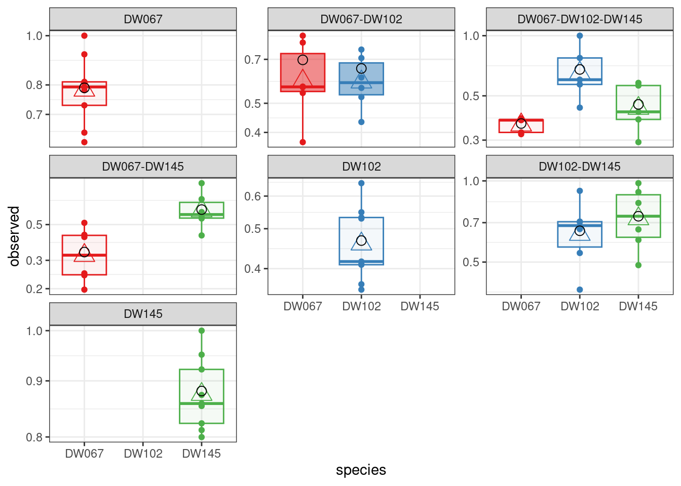
All three models are quite successful at recovering the observed means for the community we left out.
Simplified models
We have seen in the lecture that this approach estimates all \(n^2\) coefficients of the matrix \(B\). For the approach to be successful, we need to have observed enough combinations of populations growing together (each population must be present in at least \(n\) experiments with distinct compositions, each pair of populations must appear in at least one final community). When the number of populations in the pool is large, and experiments are few, this approach is unfeasible. We can therefore try to simplify the model to reduce the number of parameters.
The idea brought forward by Skwara et al. is to approximate the matrix \(B\) as the sum of a diagonal matrix and a low-rank matrix. For example, a version of the model with only \(n + 1\) parameters reads:
\[ B = D(s) + \alpha 1_n1_n^T \]
i.e., a model in which each diagonal element \(B_{ii} = s_i + \alpha\) has its own parameter (and thus can take arbitrary values), while the off-diagonals are all the same (i.e., each population has the same “mean-field” effect on all others).
A more general model using \(3 n - 1\) parameters reads:
\[ B = D(s) + u v^T \]
in which the diagonal coefficients \(B_{ii} = s_i + u_i v_i\) can take arbitrary values, while the off-diagonal elements \(B_{ij} = u_i v_j\) are constrained; the effect of species \(j\) on \(i\) depends on two values: \(v_i\) that measures how strongly species \(i\) respond to the presence of other species, and \(v_j\) that measures the magnitude of the typical effect of species \(j\). Either \(u\) or \(v\) can be taken as unitary (i.e., \(\sum_i v_i^2 = 1\)) without loss of generality, thereby bringing the total number of parameters to \(3n-1\). When the number of populations is small, this approach does not lead to big gains (e.g., for \(n=3\) we have 8 parameters instead of 9), but the reduction in parameters is substantial when \(n\) becomes larger (e.g., for the whole data set, \(n=7\), and thus we would use 20 parameters instead of 49).
Another advantage of this approach is that we can write the inverse in linear time, thereby removing the only big computational hurdle of the approach:
\[\begin{aligned} B^{-1} 1_n&= (D(s) + u v^T)^{-1}1_n\\ &= \left(D(s)^{-1} - \frac{1}{1 + v^TD(s)^{-1}u}D(s)^{-1} u v^TD(s)^{-1}\right)1_n\\ &= D(s)^{-1}\left(1_n - \frac{v^T D(s)^{-1}1_n}{1 + v^TD(s)^{-1}u} u\right) \end{aligned} \]
These models can be derived from the consumer-resource framework that you have seen in class.
We can test different versions of the simplified model. A model with only the diagonal and an extra parameter performs very poorly:
diag_a11 <- run_model(
  datafile = "Ishizawa_3_strains.csv", # csv file containing the data to be fit
  model = "diag_a11t",
  goalf = "LikLN",
  pars = NULL, # start from Identity matrix
  skipEM = TRUE, # go directly to numerical optimization
  plot_results = TRUE # plot the results
)
`mutate_if()` ignored the following grouping variables:
• Column `comm`[1] "numerical search"
[1] -22.62175
[1] -22.62175
[1] -22.62175
[1] -22.62175
[1] -22.62175
[1] -22.62175
[1] -22.62175
[1] -22.62175
[1] -22.62175
[1] -22.62175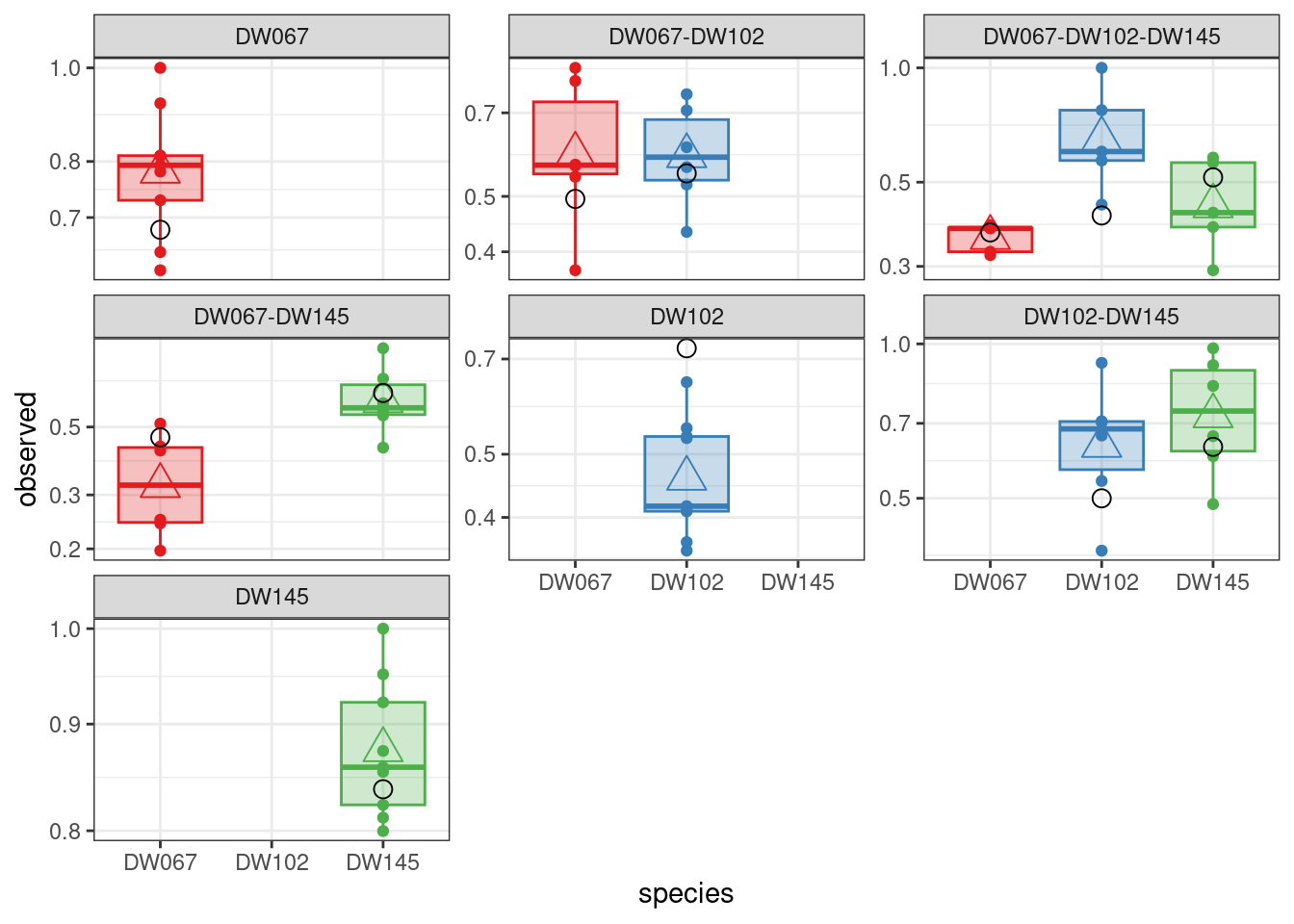
plot_pred_obs(diag_a11)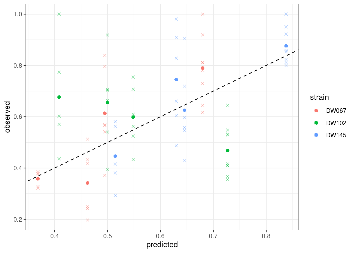
A model with symmetric interactions, \(B = D(s) + vv^T\) does slightly better:
diag_vvt <- run_model(
  datafile = "Ishizawa_3_strains.csv", # csv file containing the data to be fit
  model = "diag_vvt",
  goalf = "LikLN",
  pars = NULL, # start from Identity matrix
  skipEM = TRUE, # go directly to numerical optimization
  plot_results = TRUE # plot the results
)
`mutate_if()` ignored the following grouping variables:
• Column `comm`[1] "numerical search"
[1] -38.12933
[1] -38.36503
[1] -38.37226
[1] -38.38069
[1] -38.38508
[1] -38.39331
[1] -38.39618
[1] -38.39655
[1] -38.39655
[1] -38.39655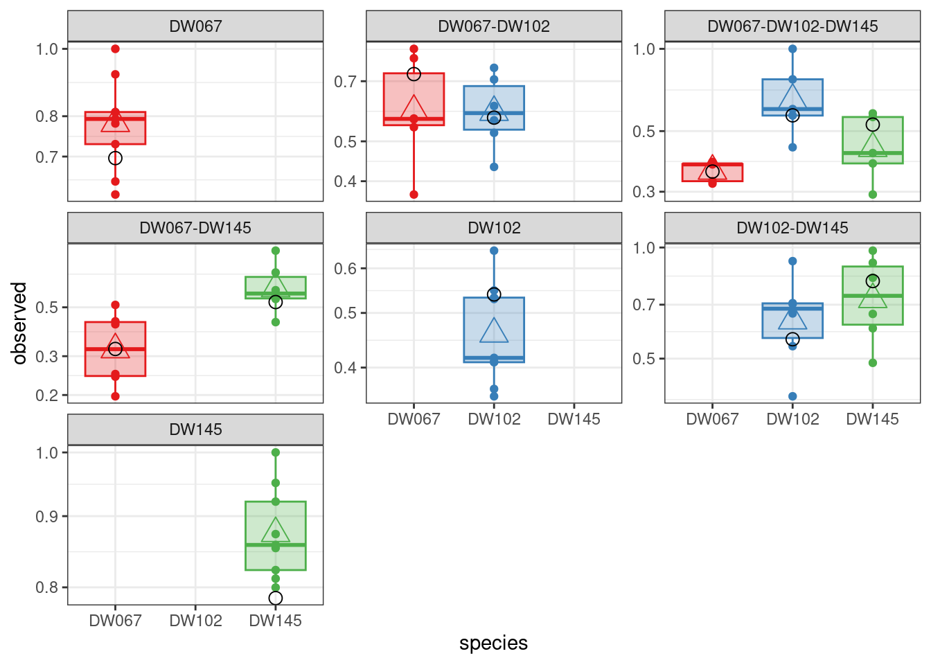
plot_pred_obs(diag_vvt)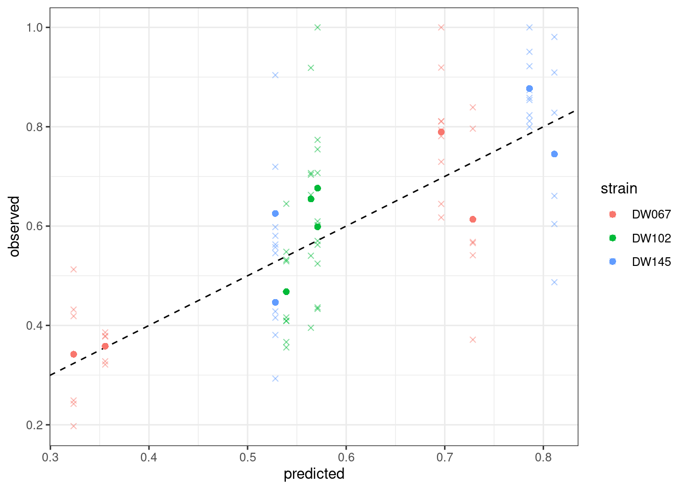
And, finally, the model with 8 parameters, \(B = D(s) + vw^T\):
A model with symmetric interactions, \(B = D(s) + vv^T\) does slightly better:
diag_vwt <- run_model(
  datafile = "Ishizawa_3_strains.csv", # csv file containing the data to be fit
  model = "diag_vwt",
  goalf = "LikLN",
  pars = NULL, # start from Identity matrix
  skipEM = TRUE, # go directly to numerical optimization
  plot_results = TRUE # plot the results
)
`mutate_if()` ignored the following grouping variables:
• Column `comm`[1] "numerical search"
[1] -34.87107
[1] -49.06619
[1] -49.06753
[1] -49.0681
[1] -49.0681
[1] -49.0681
[1] -49.0681
[1] -49.06811
[1] -49.06811
[1] -49.06811
plot_pred_obs(diag_vwt)